Stagnation point flow

In fluid dynamics, stagnation point flow represents the flow of a fluid in the immediate neighborhood of a solid surface. As the fluid approaches the surface it divides into two streams. Although the fluid is stagnant everywhere on the solid surface due to no-slip condition, the name stagnation point refers to the stagnation points of inviscid Euler solutions.

Hiemenz flow^[1][2]Edit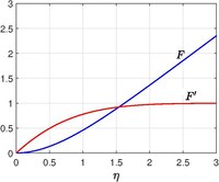

Two-dimensional stagnation point flow

Hiemenz^[3] formulated the problem and calculated the solution numerically in 1911 and subsequently by Leslie Howarth (1934).^[4] The flow in the neighborhood of the stagnation point can be modeled by a flow towards an infinite flat plate, even though the whole body is a curved one (local curvature effects are negligible). Let the plate be in the ${\displaystyle xz}$ plane with ${\displaystyle (x,y)=(0,0)}$ representing the stagnation point. The inviscid stream function ${\displaystyle \psi }$ and velocity ${\displaystyle (u,v)}$ from Potential flow theory are

${\displaystyle \psi =kxy,\quad u=kx,\quad v=-ky}$

where ${\displaystyle k}$ is an arbitrary constant (represents strain rate in the counter flow setup). For real fluid (including viscous effects), there exists a self-similar solution if one defines

${\displaystyle \eta ={\sqrt {\frac {k}{\nu }}}y,\quad \psi ={\sqrt {\nu k}}xF(\eta )}$

where ${\displaystyle \nu }$ is the Kinematic viscosity and ${\displaystyle \delta ={\sqrt {\nu /k}}}$ is a boundary layer thickness but it is constant (vorticity generated at the solid surface is prevented diffusing far away by an opposing convection, similar profiles are Blasius boundary layer with suction, Von Kármán swirling flow etc.,). Then the velocity components and subsequently pressure and the equation for ${\displaystyle F(\eta )}$ using Navier–Stokes equations are

${\displaystyle u=kxF',\quad v=-{\sqrt {\nu k}}F,\quad {\frac {p_{o}-p}{\rho }}={\frac {1}{2}}k^{2}x^{2}+k\nu F'+{\frac {1}{2}}k\nu F^{2}}$

${\displaystyle F'''+FF''-F'^{2}+1=0}$

and the boundary condition due to no penetration and no-slip and the free stream condition for ${\displaystyle u}$ (Note boundary conditions for ${\displaystyle v}$ far away from the plate is not specified, because it is part of the solution - a typical boundary layer problem) are

${\displaystyle F(0)=0,\ F'(0)=0,F'(\infty )=1.}$

The problem formulated here is the special case of Falkner-Skan boundary layer. The asymptotic forms for large ${\displaystyle \eta \rightarrow \infty }$ are

${\displaystyle F\sim \eta -0.6479,\quad u\sim kx,\quad v\sim -k(y-\delta ^{*}),\quad \delta ^{*}=0.6479\delta }$

where ${\displaystyle \delta ^{*}}$ is the displacement thickness.

Stagnation point flow with translating plate^[5]Edit

Stagnation point flow with moving plate with constant velocity ${\displaystyle U}$ can be considered as model for rotating solids near the stagnation points. The stream function is

${\displaystyle \psi ={\sqrt {\nu k}}xF(\eta )+U\delta \int _{0}^{\eta }G(\eta )d\eta }$

where ${\displaystyle G(\eta )}$ satisfies the equation

${\displaystyle G''+FG'-F'G=0,\quad G(0)=1,\quad G(\infty )=0}$

and Rott (1956)^[6] gave the solution as ${\displaystyle G(\eta )={\frac {F''(\eta )}{F''(0)}}.}$

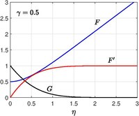
Oblique stagnation point flowEdit

The previous analyses assumes the flow impinges in normal direction. The inviscid stream function for oblique stagnation point flow is obtained by adding a constant vorticity ${\displaystyle -\zeta _{o}}$.

${\displaystyle \psi =kxy+{\frac {1}{2}}\zeta _{o}y^{2}}$

The corresponding analysis for viscous fluid is studied by Stuart (1959),^[7] Tamada (1979)^[8] and Dorrepaal (1986).^[9] The self-similar stream function is,

${\displaystyle \psi ={\sqrt {\nu k}}xF(\eta )+\zeta _{o}\delta ^{2}\int _{0}^{\eta }H(\eta )d\eta }$

where ${\displaystyle H(\eta )}$ satisfies the equation

${\displaystyle H''+FH'-F'H=0,\quad H(0)=0,\quad H'(\infty )=1}$.

Homann flowEdit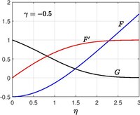

Homann flow with injection

Homann flow with suction

The corresponding problem in axisymmetric coordinate is solved by Homann (1936)^[10] and this serves a model for flow around near the stagnation point of a sphere. Paul A. Libby (1974)^[11](1976)^[12] considered Homann flow with constantly moving plate with velocity ${\displaystyle U}$ and also allowed for suction/injection with velocity ${\displaystyle V}$ at the surface.

The self-similar solution is obtained by introducing following transformation for the velocity ${\displaystyle (v_{r},v_{\theta },v_{z})}$ in cylindrical coordinates

${\displaystyle \eta ={\sqrt {\frac {k}{\nu }}}z,\quad \gamma =-{\frac {V}{2{\sqrt {k\nu }}}},\quad v_{r}=krF'(\eta )+U\cos \theta G(\eta ),\quad v_{\theta }=-U\sin \theta G(\eta ),\quad v_{z}=-2{\sqrt {k\nu }}F(\eta )}$

and the pressure is given by

${\displaystyle {\frac {p-p_{o}}{\rho }}=-{\frac {1}{2}}k^{2}r^{2}-2k\nu (F^{2}+F')}$

Therefore, the Navier–Stokes equations reduce to

${\displaystyle {\begin{aligned}F'''+2FF''-F'^{2}+1&=0,\\G''+2FG'-F'G&=0\end{aligned}}}$

with boundary conditions,

${\displaystyle F(0)=\gamma ,\quad F'(0)=0,\quad F'(\infty )=1,\quad G(0)=1,\quad G(\infty )=0.}$

When ${\displaystyle U=V=0}$, the classical Homann problem is recovered.

Plane counterflowsEdit

Jets emerging from a slot-jets creates stagnation point in between according to potential theory. The flow near the stagnation point can by studied using self-similar solution. This setup is widely used in combustion experiments. The initial study of impinging stagnation flows are due to C.Y. Wang.^[13][14] Let two fluids with constant properties denoted with suffix ${\displaystyle 1({\text{top}}),\ 2({\text{bottom}})}$ flowing from opposite direction impinge, and assume the two fluids are immiscible and the interface (located at ${\displaystyle y=0}$) is planar. The velocity is given by

${\displaystyle u_{1}=k_{1}x,\quad v_{1}=-k_{1}y,\quad u_{2}=k_{2}x,\quad v_{2}=-k_{2}y}$

where ${\displaystyle k_{1},\ k_{2}}$ are strain rates of the fluids. At the interface, velocities, tangential stress and pressure must be continuous. Introducing the self-similar transformation,

${\displaystyle \eta _{1}={\sqrt {\frac {\nu _{1}}{k_{1}}}}y,\quad u_{1}=k_{1}xF_{1}',\quad v_{1}=-{\sqrt {\nu _{1}k_{1}}}F_{1}}$

${\displaystyle \eta _{2}={\sqrt {\frac {\nu _{2}}{k_{2}}}}y,\quad u_{2}=k_{2}xF_{2}',\quad v_{2}=-{\sqrt {\nu _{2}k_{2}}}F_{2}}$

results equations,

${\displaystyle F_{1}'''+F_{1}F_{1}''-F_{1}'^{2}+1=0,\quad {\frac {p_{o1}-p_{1}}{\rho _{1}}}={\frac {1}{2}}k_{1}^{2}x^{2}+k_{1}\nu _{1}F_{1}'+{\frac {1}{2}}k_{1}\nu _{1}F_{1}^{2}}$

${\displaystyle F_{2}'''+F_{2}F_{2}''-F_{2}'^{2}+1=0,\quad {\frac {p_{o2}-p_{2}}{\rho _{2}}}={\frac {1}{2}}k_{2}^{2}x^{2}+k_{2}\nu _{2}F_{2}'+{\frac {1}{2}}k_{2}\nu _{2}F_{2}^{2}.}$

The no-penetration condition at the interface and free stream condition far away from the stagnation plane become

${\displaystyle F_{1}(0)=0,\quad F_{1}'(\infty )=1,\quad F_{2}(0)=0,\quad F_{2}'(-\infty )=1.}$

But the equations require two more boundary conditions. At ${\displaystyle \eta =0}$, the tangential velocities ${\displaystyle u_{1}=u_{2}}$, the tangential stress ${\displaystyle \rho _{1}\nu _{1}\partial u_{1}/\partial y=\rho _{2}\nu _{2}\partial u_{2}/\partial y}$ and the pressure ${\displaystyle p_{1}=p_{2}}$ are continuous. Therefore,

${\displaystyle {\begin{aligned}k_{1}F_{1}'(0)&=k_{2}F_{2}'(0),\\\rho _{1}{\sqrt {\nu _{1}k_{1}^{3}}}F_{1}''(0)&=\rho _{2}{\sqrt {\nu _{2}k_{2}^{3}}}F_{2}''(0),\\p_{o1}-\rho _{1}\nu _{1}k_{1}F_{1}'(0)&=p_{o2}-\rho _{2}\nu _{2}k_{2}F_{2}'(0).\end{aligned}}}$

where ${\displaystyle \rho _{1}k_{1}^{2}=\rho _{2}k_{2}^{2}}$ (from outer inviscid problem) is used. Both ${\displaystyle F_{i}'(0),F_{i}''(0)}$ are not known apriori, but derived from matching conditions. The third equation is determine variation of outer pressure ${\displaystyle p_{o1}-p_{o2}}$ due to the effect of viscosity. So there are only two parameters, which governs the flow, which are

${\displaystyle \Lambda ={\frac {k_{1}}{k_{2}}}=\left({\frac {\rho _{2}}{\rho _{1}}}\right)^{1/2},\quad \Gamma ={\frac {\nu _{2}}{\nu _{1}}}}$

then the boundary conditions become

${\displaystyle F_{1}'(0)=\Lambda F_{2}'(0),\quad F_{1}''(0)={\sqrt {\frac {\Gamma }{\Lambda }}}F_{2}''(0)}$.

Constant density and constant viscosityEdit

When densities and viscosities of the two impinging jets are same and constant, then the strain rate is also constant ${\displaystyle k_{1}=k_{2}=k}$ and the potential flow solution become the solution of the Navier-Stokes equations, i.e.,

${\displaystyle u=kx,\quad v=-ky}$

everywhere in the flow domain. Kerr and Dold found additional new solution called as Kerr–Dold vortex of Navier-Stokes equations in 1994 in the form of periodic array of steady vortices superposed on the constant density and constant viscosity counterflowing jets. 

This article uses material from the Wikipedia article  Metasyntactic variable, which is released under the  Creative Commons Attribution-ShareAlike 3.0 Unported License.